Archive for January, 2013

Displaying 3-D structures in the blog – a request for conversation

With the recent disclosure of a major security hole in Java, I have been wondering if perhaps my continued use of the Jmol utility for displaying 3-D molecular structures makes sense. Perhaps it is time to consider alternatives. (Right now if you click on a molecule image in one of my blog posts and you are using Firefox, a big warning sign comes up first requiring the user to actively decide to invoke the Jmol viewer. Might this warning be enough to discourage some users?)

In addition, the increasing use of mobile devices, which most often are not Java-enabled, suggests that moving to a new display option is warranted.

So, I am asking the community to participate in a conversation about how we might best address this issue in the (near) future. Is a Javascript widget the way to go? If so, which current program are people happy with? Or should we move to an HTML5 approach? And if this is the way to go, what tools are people suggesting?

If you want to see some fine examples of all three approaches (Java-based: Jmol, Javascipt-based: Chemdoodle, and HTML5-based: GLMol) I strongly encourage you to read Henry Rzepa’s recent brilliant article in Journal of Cheminformatics (DOI: 10.1186/1758-2946-5-6). This is a fantastic article to compare the old-school publication technology (as presented in modern day PDF form) and new-school enabled technology (what Henry calls a datument). First download the pdf version and read it, and then access the HTML version; I guarantee you will be impressed by the difference in the experience.

So, please chime in on what molecular viewers I might adopt for this blog, and perhaps we as a community might be able to encourage the use of and further the development of these enhanced publication technologies.

E-publishing Steven Bachrach 24 Jan 2013 3 Comments

Covalently linked cycloparaphenylenes – onwards to nanotubes

Nanotubes are currently constructed in ways that offer little control of their size and chirality. The recent synthesis of cycloparaphenylenes (CPP) provides some hope that fully controlled synthesis of nanotubes might be possible in the near future. Jasti has now made an important step forward in preparing dimers of CPP such as 1.1


1


2

They also performed B3LYP-D/6-31G(d,p) computations on 1 and the directly linked dimer 2. The optimized geometries of these two compounds in their cis and trans conformations are shown in Figure 1. Interestingly, both compounds prefer to be in the cis conformation; cis1 is 10 kcal mol-1 more stable than trans1 and cis2 is 30 kcal mol-1 more stable than the trans isomer. While a true transition state interconnecting the two isomers was not located, a series of constrained optimizations to map out a reaction surface suggests that the
barrier for 1 is about 13 kcal mol-1. The authors supply an interesting movie of this pseudo-reaction path (download the movie).

cis1

trans1

cis2

trans2

Figure 1. B3LYP-D/6-31G(d,p) optimized geometries of the cis and trans conformers of 1 and 2. (Be sure to click on these images to launch a 3-D viewer; these structures come to life in 3-D!)

References

(1) Xia, J.; Golder, M. R.; Foster, M. E.; Wong, B. M.; Jasti, R. "Synthesis, Characterization, and Computational Studies of Cycloparaphenylene Dimers," J. Am. Chem. Soc. 2012, 134, 19709-19715, DOI: 10.1021/ja307373r.

InChIs

1: InChI=1S/C106H82/c1-5-13-79-21-9-17-76-29-37-85(38-30-76)95-59-63-98(64-60-95)103-71-69-101(82(16-8-4)24-12-20-77-27-35-84(36-28-77)90-51-55-94(56-52-90)91-45-41-86(79)42-46-91)73-105(103)99-65-67-100(68-66-99)106-74-102-70-72-104(106)97-61-57-88(58-62-97)81(15-7-3)23-10-18-75-25-33-83(34-26-75)89-49-53-93(54-50-89)92-47-43-87(44-48-92)80(14-6-2)22-11-19-78-31-39-96(102)40-32-78/h5-16,21-74H,1-4,17-20H2/b21-9-,22-11-,23-10-,24-12-,79-13+,80-14+,81-15+,82-16+
InChIKey=WFVBBCVHFBTQRK-VPGVYKRGSA-N

2: InChI=1S/C100H78/c1-5-13-75-21-9-17-72-29-37-81(38-30-72)91-59-63-94(64-60-91)97-67-65-95(78(16-8-4)24-12-20-73-27-35-80(36-28-73)86-51-55-90(56-52-86)87-45-41-82(75)42-46-87)69-99(97)100-70-96-66-68-98(100)93-61-57-84(58-62-93)77(15-7-3)23-10-18-71-25-33-79(34-26-71)85-49-53-89(54-50-85)88-47-43-83(44-48-88)76(14-6-2)22-11-19-74-31-39-92(96)40-32-74/h5-16,21-70H,1-4,17-20H2/b21-9-,22-11-,23-10-,24-12-,75-13+,76-14+,77-15+,78-16+
InChIKey=HOODCSIDKUJYKE-XJQPCHFNSA-N

Uncategorized Steven Bachrach 22 Jan 2013 No Comments

A computationally inexpensive approach to correcting for BSSE

Basis set superposition error plagues all practical computations. This error results from the use of incomplete basis sets (thus pretty much all computations will suffer from this problem). The primary example of this error is in the formation of a supermolecule AB from the monomers A and B. Superposition occurs when in the computation of the supermolecule, basis functions centered on B are used to supplement the basis set of A, not to describe the bonding or interaction between the two monomers, but simply to better the description of the monomer A itself. Thus, BSSE always serves to increase the binding in the supermolecule. Recently, this concept has been extended to intramolecular BSSE, as discussed in these posts (A and B).

The counterpoise correction proposed by Boys and Bernardi corrects for the superposition by computing the energy of each monomer using the basis sets centered on both monomers, often referred to as ghost orbitals because the functions are used but not the nuclei upon which they are centered. This can overcorrect for superposition but is the only widely utilized approach to treat the problem. A variation on this approach is what has been suggested for the intramolecular
BBSE problem.

A major discouragement for wider use of counterpoise correction is its computational cost. Kruse and Grimme offer a semi-empirical approach that is extremely cost effective and appears to strongly mimic the traditional counterpoise correction.1

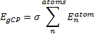
They define the geometric counterpoise scheme (gCP) that provides an energy correction EgCP that can be added onto the electronic energy. This term is defined as

Eq. (1)

where σ is an empirically fitted scaling term. The atomic contributions are defined as

Eq. (2)

where emiss are the errors in the energy of an atom with a particular target basis set, relative to the energy with some large basis set:

Eq. (3)

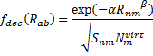
(On a technical matter, the atomic terms are computed in an electric field of 0.6a.u. in order to get some population into higher energy orbitals.) The fdec term is a decay function that relates to the distance between the atoms (Rnm) and the overlap
(Snm):

Eq. (4)

where Nvirt is the number of virtual orbitals on atom m, and α and β are fit parameters. Lastly, the overlap term comes from the integral of a single Slater orbital with coefficient

ξ = η(ξs + ξp)/2

Eq. (5)

where ξs and ξp are optimized Slater exponents from extended Huckel theory, and η is the last parameter that needs to be fit.

There are four parameters and these need to be fit for each specific combination of method (functional) and basis set. Kruse and Grimme provide parameters for a number of combinations, and suggest that the parameters devised for B3LYP are suitable for other functionals.

So what is this all good for? They demonstrate that for a broad range of benchmark systems involving weak bonds, the that gCP corrected method coupled with the DFT-D3 dispersion correction provides excellent results, even with B3LYP/6-31G*! This allows one to potentially run a computation on very large systems, like proteins, where large basis sets, like TZP or QZP, would be impossible. In a follow-up paper,2 they show that the B3LYP/6-31G*-gCP-D3 computations of a few Diels-Alder reactions and computations of strain energies of fullerenes match up very well with computations performed at significantly higher levels.

Once this gCP method and the D3 correction are fully integrated within popular QM programs, this combined methodology should get some serious attention. Even in the absence of this integration, these energy corrections can be obtained using the web service provided by Grimme at http://www.thch.uni-bonn.de/tc/gcpd3.

References

(1) Kruse, H.; Grimme, S. "A geometrical correction for the inter- and intra-molecular basis set superposition error in Hartree-Fock and density functional theory calculations for large systems," J. Chem. Phys 2012, 136, 154101-154116, DOI: 10.1063/1.3700154

(2) Kruse, H.; Goerigk, L.; Grimme, S. "Why the Standard B3LYP/6-31G* Model Chemistry Should Not Be Used in DFT Calculations of Molecular Thermochemistry: Understanding and Correcting the Problem," J. Org. Chem. 2012, 77, 10824-10834, DOI: 10.1021/jo302156p

BSSE &Grimme Steven Bachrach 15 Jan 2013 No Comments

Benchmarked Dispersion corrected DFT and SM12

This is a short post mainly to bring to the reader’s attention a couple of recent JCTC papers.

The first is a benchmark study by Hujo and Grimme of the geometries produced by DFT computations that are corrected for dispersion.1 They use the S22 and S66 test sets that span a range of compounds expressing weak interactions. Of particular note is that the B3LYP-D3 method provided the best geometries, suggesting that this much (and justly) maligned functional can be significantly improved with just the simple D3 fix.

The second paper entails the description of Truhlar and Cramer’s latest iteration on their solvation model, namely SM12.2 The main change here is the use of Hirshfeld-based charges, which comprise their Charge Model 5 (CM5). The training set used to obtain the needed parameters is much larger than with previous versions and allows for treating a very broad set of solvents. Performance of the model is excellent.

References

(1) Hujo, W.; Grimme, S. "Performance of Non-Local and Atom-Pairwise Dispersion Corrections to DFT for Structural Parameters of Molecules with Noncovalent Interactions," J. Chem. Theor. Comput. 2013, 9, 308-315, DOI: 10.1021/ct300813c

(2) Marenich, A. V.; Cramer, C. J.; Truhlar, D. G. "Generalized Born Solvation Model SM12," J. Chem. Theor. Comput. 2013, 9, 609-620, DOI: 10.1021/ct300900e

Cramer &DFT &Grimme &Solvation &Truhlar Steven Bachrach 14 Jan 2013 No Comments

Long C-O bonds

I have written a number of posts discussing long C-C bonds (here and here). What about very long bonds between carbon and a heteroatom? Well, Mascal and co-workers1 have computed the structures of some oxonium cations that express some very long C-O bonds. The champion, computed at MP2/6-31+G**, is the oxatriquinane 1, whose C-O bond is predicted to be 1.602 Å! (It is rather disappointing that the optimized structures are not included in the supporting materials!) The long bond is attributed not to dispersion forces, as in the very long C-C bonds (see the other posts), but rather to σ(C-H) or σ(C-C) donation into the σ*(C-O) orbital.


1

Inspired by these computations, they went ahead and synthesized 1 and some related species. They were able to get crystals of 1 as a (CHB11Cl11) salt. The experimental C-O bond lengths for the x-ray crystal study are 1.591, 1.593, and 1.622 Å, confirming the computational prediction of long C-O bonds.

As an aside, they also noted many examples of very long C-O distances within the Cambridge
Structural database that are erroneous – a cautionary note to anyone making use of this database to identify unusual structures.

References

(1) Gunbas, G.; Hafezi, N.; Sheppard, W. L.; Olmstead, M. M.; Stoyanova, I. V.; Tham, F. S.; Meyer, M. P.; Mascal, M. "Extreme oxatriquinanes and a record C–O bond length," Nat. Chem. 2012, 4, 1018-1023, DOI: 10.1038/nchem.1502

InChIs

1: InChI=1S/C21H39O/c1-16(2,3)19-10-12-20(17(4,5)6)14-15-21(13-11-19,22(19)20)18(7,8)9/h10-15H2,1-9H3/q+1/t19-,20+,21-
InChIKey=VTBHIDVLNISMTR-WKCHPHFGSA-N

Uncategorized Steven Bachrach 07 Jan 2013 1 Comment